(Beta) Problem Set 2: Tax Regression

The questions below are due on Friday May 09, 2025; 05:00:00 PM.
 

Download Files

1) Intro

1.1) Pset Beta-Testing Info

Thank you so much for beta-testing the psets that we'll be using for the new and improved version of 6.100A/B in the fall! A few important notes:

• As soon as you see this, if you will be beta-testing this pset please drop your kerb in this form. Do it right now please!! This is so that if I discover mistakes in the pset and need to let you know about it, I can email you.
• Along those lines, if you discover mistakes or ambiguities in the pset that make it difficult to complete the pset properly, feel free to let me know at abbychou@mit.edu.
• If you're a 6.100L student, you can get a few extra credit points for doing either this pset and/or the beta of pset 2. To get credit, you must come to my (Abby's) OH (see below) and do a checkoff with me BEFORE the pset due date of 5pm on Friday, May 9.
• Checkoffs and Office Hours: I (abby) will be running all help and checkoffs for the beta-tested psets, so you won't be able to get help during all of the normal 6.100 office hour times. Here is a gcal that tells you when I'll be at OH, so you can get help and/or do your checkoff! Just come to the normal OH room but don't bother hopping on the queue: just look for me (I am an asian gal with very long hair).
• As you work, please record how long it takes you to complete each section of the pset.
• Also please jot down anything you found confusing, plus anything that might be difficult for new programmers. Before seeing this pset, we will have taught the 6.1000 students variables/basic python syntax, loops, tuples and lists (but NOT list comprehensions or dictionaries), functions, and linear regression.

1.2) Introduction

Some states, such as California, allow municipalities (local city/town governments) to impose a sales tax. The City Council of Beaver City decided to raise their tax rate. They had tried multiple rates already, and discovered that the higher the rate, the higher the revenue, as shown below:

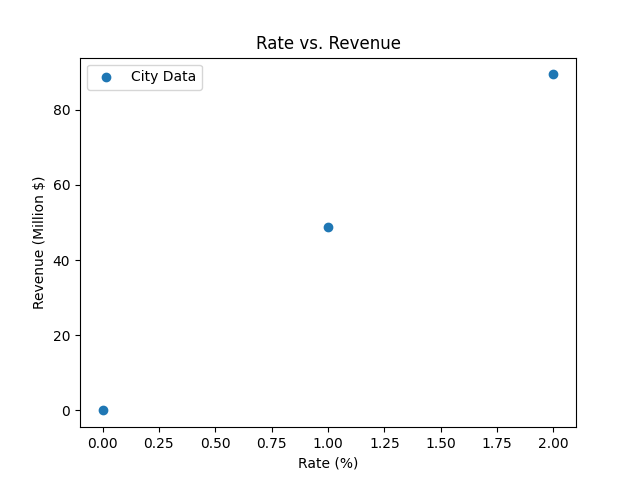
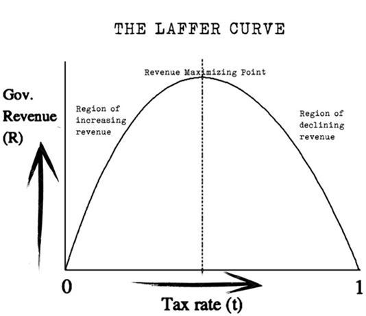
One executive argued that revenue seemed to going up almost linearly with price, and therefore there was no limit on what they could charge. Another executive argued that some academic theories predict a quadratic trend—revenue would go up for a while than start to drop as the higher rate led to less local shopping.

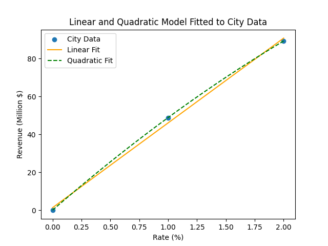
They decided to fit both a linear and a quadratic curve to the existing data, and see what each model predicts at different rates.

1.3) File setup

Download the file beta_ps2.zip and extract all files to the same directory. The files included are:

• ps2.py: This is the main file where you will implement your pset! Your code will not be autograded: your plots and code will be graded manually by the staff who does your checkoff (and our handgraders may give a second look). As such, you can modify ps2.py as much as you wish, and you should write at least 2 of your own functions to avoid repetition and/or organize your code.

Note: since your solution will not be autograded, you will be asked to run your code and show the plots it generates during your checkoff.

1.4) Important Note

For this pset, you should be using matplotlib to generate the plots. The data is provided for you in ps2.py. You should NOT use numpy or any other library besides matplotlib. If you're unsure how to implement anything, google and the matplotlib documentation are your friends!

2) Rate vs. Revenue Data

Produces a plot that shows rate versus revenue. It should look like this plot (the same as above):

3) Fitting Models

First, use a guess and check algorithm to fit a linear and a quadratic model to the lists (you may not use numpy or any other tool that fits a polynomial). Assume that for the linear model, the slope m is between 0 and 100, and the y-intercept b is between -10 and 10. Assume that for the quadratic model ax**2 + bx + c, a is between –5 and 0 (it has to be non-positive because the parabola is concave), b is between 0 and 250, and c is between 0 and 10. (We just chose numbers that encompass what's reasonable for the coefficients to be, based on what the data looks like.) You should be finding the linear/quadratic equation that minimizes MSE, as in typical linear regression.

Then, produce a plot that shows the original data and the two models. It should be labeled, and look something like:

4) Predicted Revenue

Now, the city needs to predict how much tax revenue they would collect if they increased rates beyond the 0%, 1%, and 2% rates they've already tried.

For this section, produce a plot that shows the predicted revenues of the linear and quadratic model for rates ranging from 0% to 9%. It should look something like this:

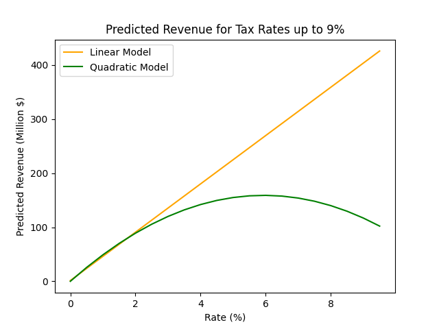
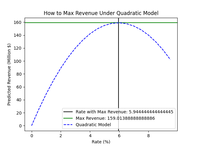
5) Finding Max Revenue

Looking at the plots, the city government decides that the quadratic model is probably the more accurate one. They ask you to use it to determine the tax rate that will maximize their revenue.

Produce a new plot that shows the predicted revenues of only the quadratic model for rates ranging from 0 to 9%. It should include a horizontal line indicating the maximum revenue and a vertical line indicating the rate that achieves that revenue, and should have the numerical values of the maximum (rate and predicted revenue) in the legend of the plot. It should look something like the following, but the aesthetic doesn't need to match exactly.

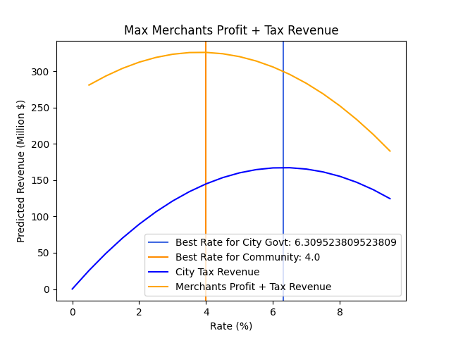
6) Optional: Balancing the Merchant's Interests

When the City Council held a meeting to propose that the rate be raised to 6%, the merchants complained. They pointed out that maximizing the revenue to the city would reduce the merchant’s revenue and thus profit. Using the quadratic model, produce a plot that shows the relationship of tax rate to (the merchants' profit + the revenue collected by the city). Hint: you can use the tax revenue and tax rate to infer the total sales revenue, and infer the profit from the total sales revenue, assuming a 5% profit margin.

To compare this result with the rate that just maximizes the city's revenue, mark both the optimal rate for the city and optimal rate for the city and merchants combined on the graph. It might look something like the following.

7) Hand-in procedure

Submit your code on the website here, but it will not be autograded. You will be asked to run your code during your checkoff, and we'll visually check that it produces the correct plots as we ask you to explain your code.

7.1) Time info

How long did this problem set take you to complete? Please answer in hours.

Loading...

7.2) Submission

It will say error: cannot autograde your code. Don't worry about this!

Select File No file selected

Loading...